Python算法设计篇(7)

Python算法设计篇(7) Chapter 7: Greed is good? Prove it!

It’s not a question of enough, pal.
——Gordon Gekko, Wall Street

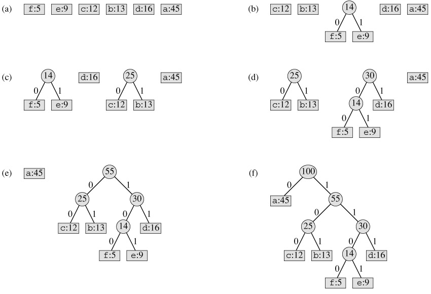
本节主要通过几个例子来介绍贪心策略，主要包括背包问题、哈夫曼编码和最小生成树

贪心算法顾名思义就是每次都贪心地选择当前最好的那个(局部最优解)，不去考虑以后的情况，而且选择了就不能够“反悔”了，如果原问题满足贪心选择性质和最优子结构，那么最后得到的解就是最优解。贪心算法和其他的算法比较有明显的区别，动态规划每次都是综合所有子问题的解得到当前的最优解(全局最优解)，而不是贪心地选择；回溯法是尝试选择一条路，如果选择错了的话可以“反悔”，也就是回过头来重新选择其他的试试。

这个算法想必大家也都很熟悉了，我觉得贪心法总是比较容易想到，但是很难证明它是正确的，所有对于一类问题，条件稍有不同也许就不能使用贪心策略了。这一节采用类似上节的形式，记录下原书中的一些重点难点内容

[果然贪心我领悟的不够，很多问题我貌似都讲不到点子上，大家将就着看下]

1.匹配问题 matching problem (maximum-weight matching problem)

问题是这样的，有一群人打算一起跳探戈，跳之前要进行分组，一个男人和一个女人成为一组，而且任意一个异性组合都会一个相应的匹配值(compatibility)，目标是求使得匹配值之和达到最大的分组方式。

To be on the safe side, just let me emphasize that this greedy solution would not work in general, with an arbitrary set of weights. The distinct powers of two are key here.

一般情况下，如果匹配值是任意值的话，这个问题使用贪心法是不行的！但是如果匹配值都是2的整数幂的话，那么贪心法就能解决这个问题了！[这点我不明白，这是此题的一个重点，避免误导，我附上原文，不解释了，如果读者有明白了的希望能留言告知，嘿嘿]

In this case (or the bipartite case, for that matter), greed won’t work in general. However, by some freak coincidence, all the compatibility numbers happen to be distinct powers of two. Now, what happens?

Let’s first consider what a greedy algorithm would look like here and then see why it yields an optimal result. We’ll be building a solution piece by piece—let the pieces be pairs and a partial solution be a set of pairs. Such a partial solution is valid only if no person in it participates in two (or more) of its pairs. The algorithm will then be roughly as follows:

1. List potential pairs, sorted by decreasing compatibility.

2. Pick the first unused pair from the list.

3. Is anyone in the pair already occupied? If so, discard it; otherwise, use it.

4. Are there any more pairs on the list? If so, go to 2.

As you’ll see later, this is rather similar to Kruskal’s algorithm for minimum spanning trees (although that works regardless of the edge weights). It also is a rather prototypical greedy algorithm. Its correctness is another matter. Using distinct powers of two is sort of cheating, because it would make virtually any greedy algorithm work; that is, you’d get an optimal result as long as you could get a valid solution at all. Even though it’s cheating (see Exercise 7-3), it illustrates the central idea here: making the greedy choice is safe. Using the most compatible of the remaining couples will always be at least as good as any other choice.

贪心解决的思路大致如下：首先列举出所有可能的组合，然后将它们按照匹配值进行降序排序，接着按顺序从中选择前面没有使用过而且人物没有在前面出现过的组合，遍历完整个序列就得到了匹配值之和最大的分组方式。

[原书关于稳定婚姻的扩展知识 EAGER SUITORS AND STABLE MARRIAGES]

There is, in fact, one classical matching problem that can be solved (sort of) greedily: the stable marriage problem. The idea is that each person in a group has preferences about whom he or she would like to marry. We’d like to see everyone married, and we’d like the marriages to be stable, meaning that there is no man who prefers a woman outside his marriage who also prefers him. (To keep things simple, we disregard same-sex marriages and polygamy here.)

There’s a simple algorithm for solving this problem, designed by David Gale and Lloyd Shapley. The formulation is quite gender-conservative but will certainly also work if the gender roles are reversed. The algorithm runs for a number of rounds, until there are no unengaged men left. Each round consists of two steps:

1. Each unengaged man proposes to his favorite of the women he has not yet asked.

2. Each woman is (provisionally) engaged to her favorite suitor and rejects the rest.

This can be viewed as greedy in that we consider only the available favorites (both of the men and women) right now. You might object that it’s only sort of greedy in that we don’t lock in and go straight for marriage; the women are allowed to break their engagement if a more interesting suitor comes along. Even so, once a man has been rejected, he has been rejected for good, which means that we’re guaranteed progress.

To show that this is an optimal and correct algorithm, we need to know that everyone gets married and that the marriages are stable. Once a woman is engaged, she stays engaged (although she may replace her fiancé). There is no way we can get stuck with an unmarried pair, because at some point the man would have proposed to the woman, and she would have (provisionally) accepted his proposal.

How do we know the marriages are stable? Let’s say Scarlett and Stuart are both married but not to each other. Is it possible they secretly prefer each other to their current spouses? No: if so, Stuart would already have proposed to her. If she accepted that proposal, she must later have found someone she liked better; if she rejected it, she would already have a preferable mate.

Although this problem may seem silly and trivial, it is not. For example, it is used for admission to some colleges and to allocate medical students to hospital jobs. There have, in fact, been written entire books (such as those by Donald Knuth and by Dan Gusfield and Robert W. Irwing) devoted to the problem and its variations.

2.背包问题

这个问题大家很熟悉了，而且该问题的变种很多，常见的有整数背包和部分背包问题。问题大致是这样的，假设现在我们要装一些物品到一个书包里，每样物品都有一定的重量w和价值v，但是呢，这个书包承重量有限，所以我们要进行决策，如何选择物品才能使得最终的价值最大呢？整数背包是说一个物品要么拿要么不拿，比如茶杯或者台灯等等，而部分背包问题是说一个物品你可以拿其中的一部分，比如一袋子苹果放不下可以只装半袋子苹果。[更加复杂的版本是说每个物品都有一定的体积，同时书包还有体积的限制等等]

很显然，部分背包问题是可以用贪心法来求解的，我们计算每个物品的单位重量的价值，然后将它们降序排序，接着开始拿物品，只要装得下全部的该类物品那么就全装进去，如果不能全部装下就装部分进去直到书包载重量满了为止，这种策略肯定是正确的。

但是，整数背包问题就不能用贪心策略了。整数背包问题还可以分成两种：一种是每类物品数量都是有限的(bounded)，比如只有3个茶杯和2个台灯；还有一种是数量无限的(unbounded)，也就是你想要多少有多少，这两种都不能使用贪心策略。0-1背包问题是典型的第一种整数背包问题，看下算法导论上的这个例子就明白了，在(b)中，虽然物品1单位重量的价值最大，但是任何包含物品1的选择都没有超过选择物品2和物品3得到的最优解220；而(c)中能达到最大的价值是240。

整数背包问题还没有能够在多项式时间内解决它的算法，下一节我们介绍的动态规划能够解决0-1背包问题，但是是一个伪多项式时间复杂度。[实际时间复杂度是$O(nw)$，n是物品数目，w是书包载重量，严格意义上说这不是一个多项式时间复杂度]

There are two important cases of the integer knapsack problem—the bounded and unbounded cases. The bounded case assumes we have a fixed number of objects in each category,4 and the unbounded case lets us use as many as we want. Sadly, greed won’t work in either case. In fact, these are both unsolved problems, in the sense that no polynomial algorithms are known to solve them. There is hope, however. As you’ll see in the next chapter, we can use dynamic programming to solve the problems in pseudopolynomial time, which may be good enough in many important cases. Also, for the unbounded case, it turns out that the greedy approach ain’t half bad! Or, rather, it’s at least half good, meaning that we’ll never get less than half the optimum value. And with a slight modification, you can get as good results for the bounded version, too. This concept of greedy approximation is discussed in more detail in Chapter 11.

3.哈夫曼编码

这个问题原始是用来实现一个可变长度的编码问题，但可以总结成这样一个问题，假设我们有很多的叶子节点，每个节点都有一个权值w(可以是任何有意义的数值，比如它出现的概率)，我们要用这些叶子节点构造一棵树，那么每个叶子节点就有一个深度d，我们的目标是使得所有叶子节点的权值与深度的乘积之和$$\Sigma w_{i}d_{i}$$最小。

很自然的一个想法就是，对于权值大的叶子节点我们让它的深度小些(更加靠近根节点)，权值小的让它的深度相对大些，这样的话我们自然就会想着每次取当前权值最小的两个节点将它们组合出一个父节点，一直这样组合下去直到只有一个节点即根节点为止。如下图所示的示例

代码实现比较简单，使用了heapq模块，树结构是用list来保存的，有意思的是其中zip函数的使用，其中统计函数count作为zip函数的参数，详情见python docs

from heapq import heapify, heappush, heappop
from itertools import count

def huffman(seq, frq):
    num = count()
    trees = list(zip(frq, num, seq))            # num ensures valid ordering
    heapify(trees)                              # A min-heap based on freq
    while len(trees) > 1:                       # Until all are combined
        fa, _, a = heappop(trees)               # Get the two smallest trees
        fb, _, b = heappop(trees)
        n = next(num)
        heappush(trees, (fa+fb, n, [a, b]))     # Combine and re-add them
    # print trees
    return trees[0][-1]

seq = "abcdefghi"
frq = [4, 5, 6, 9, 11, 12, 15, 16, 20]
print huffman(seq, frq)
# [['i', [['a', 'b'], 'e']], [['f', 'g'], [['c', 'd'], 'h']]]

现在我们考虑另外一个问题，合并文件问题，假设我们将大小为 m 和大小为 n 的两个文件合并在一起需要 m+n 的时间，现在给定一些文件，求一个最优的合并策略使得所需要的时间最小。

如果我们将上面哈夫曼树中的叶子节点看成是文件，两个文件合并得到的大文件就是树中的内部节点，假设每个节点上都有一个值表示该文件的大小，合并得到的大文件上的值是合并的两个文件的值之和，那我们的目标是就是使得内部节点的和最小的合并方案，因为叶子节点的大小是固定的，所以实际上也就是使得所有节点的和最小的合并方案！

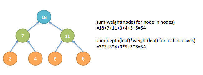
consider how each leaf contributes to the sum over all nodes: the leaf weight occurs as a summand once in each of its ancestor nodes—which means that the sum is exactly the same! That is, sum(weight(node) for node in nodes) is exactly the same as sum(depth(leaf)*weight(leaf) for leaf in leaves).

细想也就有了一个叶子节点的所有祖先节点们都有一份该叶子节点的值包含在里面，也就是说所有叶子节点的深度与它的值的乘积之和就是所有节点的值之和！可以看下下面的示例图，最终我们知道哈夫曼树就是这个问题的解决方案。

[哈夫曼树问题的一个扩展就是最优二叉搜索树问题，后者可以用动态规划算法来求解，感兴趣的话可以阅读算法导论中动态规划部分内容]

4.最小生成树

最小生成树是图中的重要算法，主要有两个大家耳熟能详的Kruskal和Prim算法，两个算法都是基于贪心策略，不过略有不同。

[如果对最小生成树问题的历史感兴趣的话作者推荐看这篇论文“On the History of the Minimum Spanning Tree Problem,” by Graham and Hell]

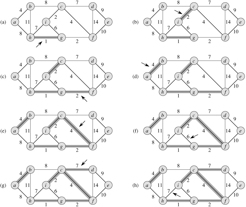
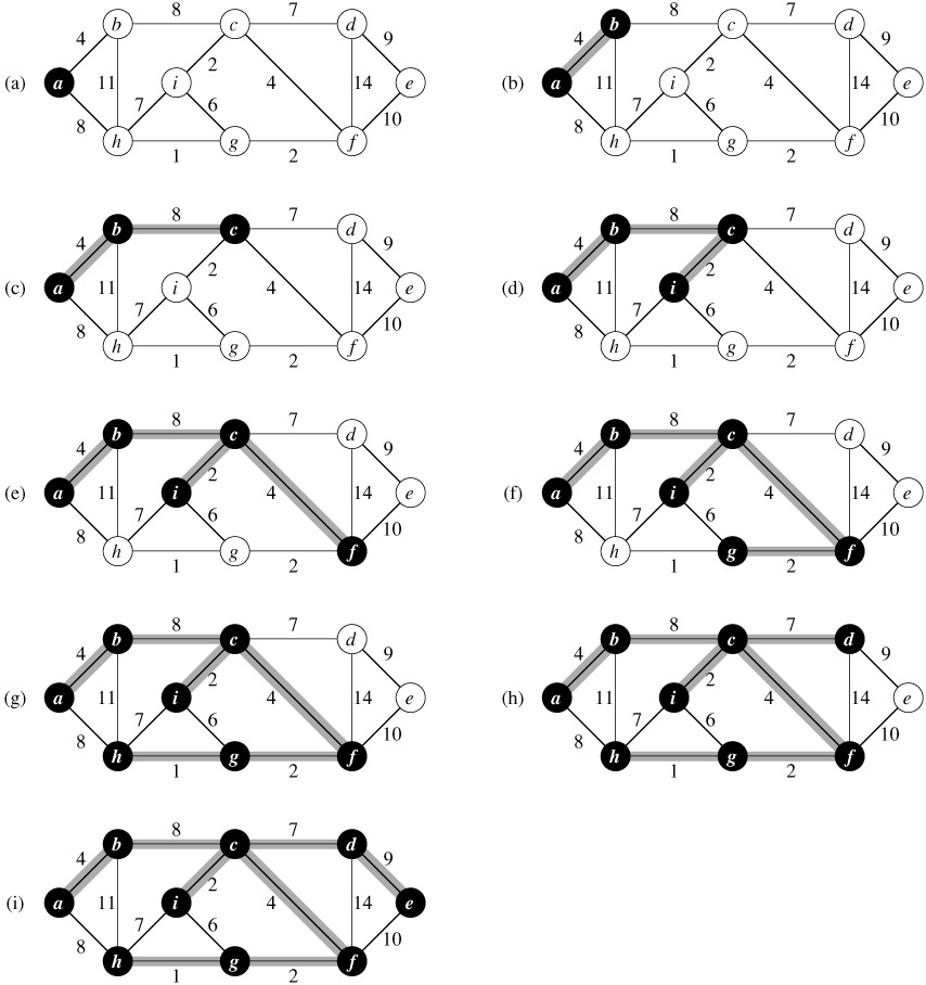
不了解Kruskal或者Prim算法的童鞋可以参考算法导论的示例图理解下面的内容

Kruskal算法

Prim算法

连通无向图G的生成树是指包含它所有顶点但是部分边的子图，假设每条边都有一个权值，那么权值之和最小的生成树就是最小生成树，它不一定是唯一的。如果图G是非连通的，那么它就没有生成树。

前面我们在介绍遍历的时候也得到过生成树，那里我们是一个顶点一个顶点进行遍历，下面我们通过每次添加一条边来得到最小生成树，而且每次我们贪心地选择剩下的边中权值最小的那条边，但是要保证不能形成环！

那怎么判断是否会出现环呢？

假设我们要考虑是否添加边(u,v)，一个最直接的想法就是遍历已生成的树，看是否能够从 u 到 v，如果能，那么就舍弃这条边继续考虑后面的边，否则就添加这条边。很显然，采用遍历的方式太费时了。

再假设我们用一个集合来保存我们已经生成的树中的节点，如果我们要考虑是否添加边(u,v)，那么我们就看下集合中这两个节点是否都存在，如果都存在的话说明这条边加进来的话会形成环。这么做可以在常数时间内确定是否会形成环，但是…它是错误的！除非我们每次添加一条边之后得到的局部解一直都只有一棵树才对，如果之前加入的节点 u 和节点 v 在不同的分支上的话，上面的判断不能确定添加这条边之后会形成环！[后面的Prim算法采用的策略就能保证局部解一直都是一棵树]

下面我们可以试着让每个加入的节点都知道自己处在哪个分支上，而且我们可以用分支中的某一个节点作为该分支的“代表”，该分支中的所有节点都指向这个“代表”，显然我们接下来会遇到分支合并的问题。如果两个分支因为某条边的加入而连通了，那么它们就要合并了，那怎么合并呢？我们让两个分支中的所有节点都指向同一个“代表”就行了，但是这是一个线性时间的操作，我们可以做得更快！假设我们改变下策略，让每个节点指向另一个节点(这个节点不一定是分支的“代表”)，如果我们顺着指向链一直找，就肯定能找到“代表”，因为“代表”是自己指向自己的。这样的话，如果两个分支要合并，只需要让其中的一个分支的“代表”指向另一个分支的“代表”就行啦！这就是一个常数时间的操作。

基于上面的思路我们就有了下面的实现

#A Naïve Implementation of Kruskal’s Algorithm
def naive_find(C, u):                           # Find component rep.
    while C[u] != u:                            # Rep. would point to itself
        u = C[u]
    return u

def naive_union(C, u, v):
    u = naive_find(C, u)                        # Find both reps
    v = naive_find(C, v)
    C[u] = v                                    # Make one refer to the other

def naive_kruskal(G):
    E = [(G[u][v],u,v) for u in G for v in G[u]]
    T = set()                                   # Empty partial solution
    C = {u:u for u in G}                        # Component reps
    for _, u, v in sorted(E):                   # Edges, sorted by weight
        if naive_find(C, u) != naive_find(C, v):
            T.add((u, v))                       # Different reps? Use it!
            naive_union(C, u, v)                # Combine components
    return T

G = {
    0: {1:1, 2:3, 3:4},
    1: {2:5},
    2: {3:2},
    3: set()
    }
print list(naive_kruskal(G)) #[(0, 1), (2, 3), (0, 2)]

从上面的分析我们可以看到，虽然合并时修改指向的操作是常数时间的，但是通过指向链的方式找到“代表”所花的时间是线性的，而这里还可以做些改进。

首先，在合并(union)的时候我们让“小”分支指向“大”分支，这样平衡了之后平均查找时间肯定有所下降，那么怎么确定分支的“大小”呢？这个可以用平衡树的方式来思考，假设我们给每个节点都设置一个权重(rank or weight)，其实重要的还是“代表”的权重，如果要合并的两个分支的“代表”的权重相等的话，在将“小”分支指向“大”分支之后，还要将“大”分支的权重加1。

其次，在查找(find)的时候我们一边查找一边修正经过的点的指向，让它直接指向“代表”，这个怎么做到呢？使用递归就行了，因为递归在找到了之后会回溯，回溯的时候就可以设置其他节点的“代表”了，这个叫做path compression技术，是Kruskal算法常用的一个技巧。

基于上面的改进就有了下面优化的Kruskal算法

#Kruskal’s Algorithm
def find(C, u):
    if C[u] != u:
        C[u] = find(C, C[u])                    # Path compression
    return C[u]

def union(C, R, u, v):
    u, v = find(C, u), find(C, v)
    if R[u] > R[v]:                             # Union by rank
        C[v] = u
    else:
        C[u] = v
    if R[u] == R[v]:                            # A tie: Move v up a level
        R[v] += 1

def kruskal(G):
    E = [(G[u][v],u,v) for u in G for v in G[u]]
    T = set()
    C, R = {u:u for u in G}, {u:0 for u in G}   # Comp. reps and ranks
    for _, u, v in sorted(E):
        if find(C, u) != find(C, v):
            T.add((u, v))
            union(C, R, u, v)
    return T

G = {
    0: {1:1, 2:3, 3:4},
    1: {2:5},
    2: {3:2},
    3: set()
    }
print list(kruskal(G)) #[(0, 1), (2, 3), (0, 2)]

接下来就是Prim算法了，它其实就是我们前面介绍的traversal算法中的一种，不同点是它对待办事项(to-do list，即前面提到的“边缘节点”，也就是我们已经包含的这些节点能够直接到达的那些节点)进行了一定的排序，我们在实现BFS时使用的是双端队列deque，此时我们只要把它改成一个优先队列(priority queue)就行了，这里选用heapq模块中的堆heap。

Prim算法不断地添加新的边(也可以说是一个新的顶点)，一旦我们加入了一条新的边，可能会导致某些原来的边缘节点到生成树的距离更加近了，所以我们要更新一下它们的距离值，然后重新调整下排序，那怎么修改距离值呢？我们可以先找到原来的那个节点，然后再修改它的距离值接着重新调整堆，但是这么做实在是太麻烦了！这里有一个巧妙的技巧就是直接向堆中插入新的距离值的节点！为什么可以呢？因为插入的新节点B的距离值比原来的节点A的距离值小，那么Prim算法添加顶点的时候肯定是先弹出堆中的节点B，后面如果弹出节点A的话，因为这个节点已经添加进入了，直接忽略就行了，也就是说我们这么做不仅很简单，而且并没有把原来的问题搞砸了。下面是作者给出的详细解释，总共三点，第三点是重复的添加不会影响算法的渐近时间复杂度

• We’re using a priority queue, so if a node has been added multiple times, by the time we remove one of its entries, it will be the one with the lowest weight (at that time), which is the one we want.

• We make sure we don’t add the same node to our traversal tree more than once. This can be ensured by a constant-time membership check. Therefore, all but one of the queue entries for any given node will be discarded.

• The multiple additions won’t affect asymptotic running time

[重新添加一次权值减小了的节点就相当于是松弛(或者说是隐含了松弛操作在里面)，Re-adding a node with a lower weight is equivalent to a relaxation，这两种方式是可以相互交换的，后面图算法中作者在实现Dijkstra算法时使用的是relax，那其实我们还可以实现带relex的Prim和不带relax的Dijkstra]

根据上面的分析就有了下面的Prim算法实现

from heapq import heappop, heappush

def prim(G, s):
    P, Q = {}, [(0, None, s)]
    while Q:
        _, p, u = heappop(Q)
        if u in P: continue
        P[u] = p
        for v, w in G[u].items():
            heappush(Q, (w, u, v)) #weight, predecessor node, node
    return P

G = {
    0: {1:1, 2:3, 3:4},
    1: {0:1, 2:5},
    2: {0:3, 1:5, 3:2},
    3: {2:2, 0:4}
    }
print prim(G, 0) # {0: None, 1: 0, 2: 0, 3: 2}

[扩展知识，另一个角度来看最小生成树 A SLIGHTLY DIFFERENT PERSPECTIVE]

In their historical overview of minimum spanning tree algorithms, Ronald L. Graham and Pavol Hell outline three algorithms that they consider especially important and that have played a central role in the history of the problem. The first two are the algorithms that are commonly attributed to Kruskal and Prim (although the second one was originally formulated by Vojtěch Jarník in 1930), while the third is the one initially described by Borůvka. Graham and Hell succinctly explain the algorithms as follows. A partial solution is a spanning forest, consisting of a set of fragments (components, trees). Initially, each node is a fragment. In each iteration, edges are added, joining fragments, until we have a spanning tree.

Algorithm 1: Add a shortest edge that joins two different fragments.

Algorithm 2: Add a shortest edge that joins the fragment containing the root to another fragment.

Algorithm 3: For every fragment, add the shortest edge that joins it to another fragment.

For algorithm 2, the root is chosen arbitrarily at the beginning. For algorithm 3, it is assumed that all edge weights are different to ensure that no cycles can occur. As you can see, all three algorithms are based on the same fundamental fact—that the shortest edge over a cut is safe. Also, in order to implement them efficiently, you need to be able to find shortest edges, detect whether two nodes belong to the same fragment, and so forth (as explained for algorithms 1 and 2 in the main text). Still, these brief explanations can be useful as a memory aid or to get the bird’s-eye perspective on what’s going on.

5.Greed Works. But When?

还是老话题，贪心算法真的很好，有时候也比较容易想到，但是它什么时候是正确的呢？

针对这个问题，作者提出了些建议和方法[都比较难翻译和理解，感兴趣还是阅读原文较好]

(1)Keeping Up with the Best

This is what Kleinberg and Tardos (in Algorithm Design) call staying ahead. The idea is to show that as you build your solution, one step at a time, the greedy algorithm will always have gotten at least as far as a hypothetical optimal algorithm would have. Once you reach the finish line, you’ve shown that greed is optimal.

(2)No Worse Than Perfect

This is a technique I used in showing the greedy choice property for Huffman’s algorithm. It involves showing that you can transform a hypothetical optimal solution to the greedy one, without reducing the quality. Kleinberg and Tardos call this an exchange argument.

(3)Staying Safe

This is where we started: to make sure a greedy algorithm is correct, we must make sure each greedy step along the way is safe. One way of doing this is the two-part approach of showing (1) the greedy choice property, that is, that a greedy choice is compatible with optimality, and (2) optimal substructure, that is, that the remaining subproblem is a smaller instance that must also be solved optimally.

[扩展知识：算法导论中还介绍了贪心算法的内在原理，也就是拟阵，贪心算法一般都是求这个拟阵的最大独立子集，方法就是从一个空的独立子集开始，从一个已经经过排序的序列中依次取出一个元素，尝试添加到独立子集中，如果新元素加入之后的集合仍然是一个独立子集的话那就加入进去，这样就形成了一个更大的独立子集，待遍历完整个序列时我们就得到最大的独立子集。拟阵的内容比较难，感兴趣不妨阅读下算法导论然后证明一两道练习题挑战下，嘻嘻]

用Python代码来形容上面的过程就是

#贪心算法的框架 [拟阵的思想]
def greedy(E, S, w):
    T = []                                      # Emtpy, partial solution
    for e in sorted(E, key=w):                  # Greedily consider elements
        TT = T + [e]                            # Tentative solution
        if TT in S: T = TT                      # Is it valid? Use it!
    return T