Python算法设计篇(2) Chapter 2: The basics
Tracey: I didn’t know you were out there.
Zoe: Sort of the point. Stealth—you may have heard of it.
Tracey: I don’t think they covered that in basic.
—— From “The Message,” episode 14 of Firefly
本节主要介绍了三个内容:算法渐近运行时间的表示方法、六条算法性能评估的经验以及Python中树和图的实现方式。
1.计算模型
图灵机模型(Turing machine): A Turing machine is a simple (abstract) device that can read from, write to, and move along an infinitely long strip of paper. The actual behavior of the machines varies. Each is a so-called finite state machine: it has a finite set of states (some of which indicate that it has finished), and every symbol it reads potentially triggers reading and/or writing and switching to a different state. You can think of this machinery as a set of rules. (“If I am in state 4 and see an X, I move one step to the left, write a Y, and switch to state 9.”)
RAM模型(random-access machine):标准的单核计算机,它大致有下面三个性质
• We don’t have access to any form of concurrent execution; the machine simply executes one instruction after the other.
计算机不能并发执行而只是按照指令顺序依次执行指令。
• Standard, basic operations (such as arithmetic, comparisons, and memory access) all take constant (although possibly different) amounts of time. There are no more complicated basic operations (such as sorting).
基本的操作都是常数时间完成的,没有其他的复杂操作。
• One computer word (the size of a value that we can work with in constant time) is not unlimited but is big enough to address all the memory locations used to represent our problem, plus an extra percentage for our variables.
计算机的字长足够大以使得它能够访问所有的内存地址。
算法的本质: An algorithm is a procedure, consisting of a finite set of steps (possibly including loops and conditionals) that solves a given problem in finite time.
the notion of running time complexity (as described in the next section) is based on knowing how big a problem instance is, and that size is simply the amount of memory needed to encode it.
[算法的运行时间是基于问题的大小,这个大小是指问题的输入占用的内存空间大小]
2.算法渐近运行时间
主要介绍了大O符号、大$\Omega$符号以及大$\Theta$符号,这部分内容网上很多资料,大家也都知道了,此处略过,可以参考wikipedia_大O符号
算法导论介绍到,对于三个符号可以做如下理解:$O$ = $\le$,$\Omega$ = $\ge$, $\Theta$ = $=$
运行时间的三种特殊的情况:最优情况,最差情况,平均情况
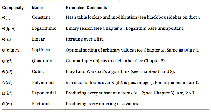
几种常见的运行时间以及算法实例 点击这里可以参考下wiki中的时间复杂度

3.算法性能评估的经验
(1)Tip 1: If possible, don’t worry about it.
如果暴力求解也还行就算了吧,别去担心了
(2)Tip 2: For timing things, use timeit.
使用timeit模块对运行时间进行分析,在使用的时候需要注意前面的运行不要影响后面的重复的运行(例如,分析排序算法运行时间,如果将前面已经排好序的序列传递给后面的重复运行是不行的)
#timeit模块简单使用实例
timeit.timeit("x = sum(range(10))")

(3)Tip 3: To find bottlenecks, use a profiler.
使用cProfile模块来获取更多的关于运行情况的内容,从而可以发现问题的瓶颈,如果系统没有cProfile模块,可以使用profile模块代替,关于这两者的更多内容可以查看Python standard library-Python Profilers
#cProfile模块简单使用实例
import cProfile
import re
cProfile.run('re.compile("foo|bar")')

#运行结果:

         194 function calls (189 primitive calls) in 0.000 seconds

   Ordered by: standard name

   ncalls  tottime  percall  cumtime  percall filename:lineno(function)
        1    0.000    0.000    0.000    0.000 <string>:1(<module>)
        1    0.000    0.000    0.000    0.000 re.py:188(compile)
        1    0.000    0.000    0.000    0.000 re.py:226(_compile)
        1    0.000    0.000    0.000    0.000 sre_compile.py:178(_compile_charset)
        1    0.000    0.000    0.000    0.000 sre_compile.py:207(_optimize_charset)
...
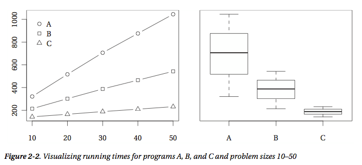
(4)Tip 4: Plot your results.
画出算法性能结果图,如下图所示,可以使用的模块有matplotlib

(5)Tip 5: Be careful when drawing conclusions based on timing comparisons.
在对基于运行时间的比较而要下结论时需要小心
First, any differences you observe may be because of random variations.
首先,你观察到的差异可能是由于输入中的随机变化而引起的
Second, there are issues when comparing averages.
其次,比较算法的平均情况下的运行时间是存在问题的[这个我未理解,以下是作者的解释]
At the very least, you should stick to comparing averages of actual timings. A common practice to get more meaningful numbers when performing timing experiments is to normalize the running time of each program, dividing it by the running time of some standard, simple algorithm. This can indeed be useful but can in some cases make your results less than meaningful. See the paper “How not to lie with statistics: The correct way to summarize benchmark results” by Fleming and Wallace for a few pointers. For some other perspectives, you could read Bast and Weber’s “Don’t compare averages,” or the more recent paper by Citron et al., “The harmonic or geometric mean: does it really matter?”
Third, your conclusions may not generalize.
最后,你的结论未必适用于一般情况 (感谢评论者@梁植华的翻译建议)
(6)Tip 6: Be careful when drawing conclusions about asymptotics from experiments.
在对从实验中得到关于渐近时间的信息下结论时需要小心,实验只是对于理论的一个支撑,可以通过实验来推翻一个渐近时间结果的假设,但是反过来一般不行 [以下是作者的解释]
If you want to say something conclusively about the asymptotic behavior of an algorithm, you need to analyze it, as described earlier in this chapter. Experiments can give you hints, but they are by their nature finite, and asymptotics deal with what happens for arbitrarily large data sizes. On the other hand, unless you’re working in theoretical computer science, the purpose of asymptotic analysis is to say something about the behavior of the algorithm when implemented and run on actual problem instances, meaning that experiments should be relevant.
4.在Python中实现树和图
[Python中的dict和set]
Python中很多地方都使用了hash策略,在前面的Python数据结构篇中的搜索部分已经介绍了hash的内容。Python提供了hash函数,例如hash("Hello, world!")得到-943387004357456228 (结果不一定相同)。Python中的dict和set都使用了hash机制,所以平均情况下它们获取元素都是常数时间的。
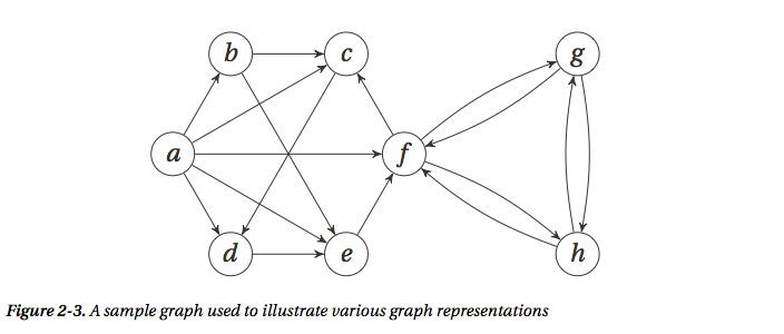
(1)图的表示:最常用的两种表示方式是邻接表和邻接矩阵 [假设要表示的图如下]

邻接表 Adjacency Lists
因为历史原因,邻接表往往都是指链表list,但实际上也可以是其他的,例如在python中也可以是set或者dict,不同的表示方式有各自的优缺点,它们判断节点的连接关系和节点的度的方式甚至两个操作的性能都不太一样。
① adjacency lists 表示形式
# A Straightforward Adjacency List Representation
a, b, c, d, e, f, g, h = range(8)
N = [
    [b, c, d, e, f],    # a
    [c, e],             # b
    [d],                # c
    [e],                # d
    [f],                # e
    [c, g, h],          # f
    [f, h],             # g
    [f, g]              # h
]

b in N[a] # Neighborhood membership -> True
len(N[f]) # Degree -> 3
② adjacency sets 表示形式
# A Straightforward Adjacency Set Representation
a, b, c, d, e, f, g, h = range(8)
N = [
    {b, c, d, e, f},    # a
    {c, e},             # b
    {d},                # c
    {e},                # d
    {f},                # e
    {c, g, h},          # f
    {f, h},             # g
    {f, g}              # h
]

b in N[a] # Neighborhood membership -> True
len(N[f]) # Degree -> 3
基本上和adjacency lists表示形式一样对吧?但是,对于list,判断一个元素是否存在是线性时间$O(N(v))$,而在set中是常数时间$O(1)$,所以对于稠密图使用adjacency sets要更加高效。
③ adjacency dicts 表示形式,这种情况下如果边是带权值的都没有问题!
# A Straightforward Adjacency Dict Representation
a, b, c, d, e, f, g, h = range(8)
N = [
    {b:2, c:1, d:3, e:9, f:4},    # a
    {c:4, e:3},                   # b
    {d:8},                        # c
    {e:7},                        # d
    {f:5},                        # e
    {c:2, g:2, h:2},              # f
    {f:1, h:6},                   # g
    {f:9, g:8}                    # h
]

b in N[a] # Neighborhood membership -> True
len(N[f]) # Degree -> 3
N[a][b] # Edge weight for (a, b) -> 2
除了上面三种方式外,还可以改变外层数据结构,上面三个都是list,其实也可以使用dict,例如下面的代码,此时节点是用字母表示的。在实际应用中,要根据问题选择最合适的表示形式。
N = {
    'a': set('bcdef'),
    'b': set('ce'),
    'c': set('d'),
    'd': set('e'),
    'e': set('f'),
    'f': set('cgh'),
    'g': set('fh'),
    'h': set('fg')
}
邻接矩阵 Adjacency Matrix
使用嵌套的list,用1和0表示点和点之间的连接关系,此时点之间的连接性判断时间是常数,但是对于度的计算时间是线性的
# An Adjacency Matrix, Implemented with Nested Lists
a, b, c, d, e, f, g, h = range(8)
N = [[0,1,1,1,1,1,0,0], # a
     [0,0,1,0,1,0,0,0], # b
     [0,0,0,1,0,0,0,0], # c
     [0,0,0,0,1,0,0,0], # d
     [0,0,0,0,0,1,0,0], # e
     [0,0,1,0,0,0,1,1], # f
     [0,0,0,0,0,1,0,1], # g
     [0,0,0,0,0,1,1,0]] # h

N[a][b] # Neighborhood membership -> 1
sum(N[f]) # Degree -> 3
如果边带有权值,也可以使用权值代替1,用inf代替0
a, b, c, d, e, f, g, h = range(8)
_ = float('inf')

W = [[0,2,1,3,9,4,_,_], # a
     [_,0,4,_,3,_,_,_], # b
     [_,_,0,8,_,_,_,_], # c
     [_,_,_,0,7,_,_,_], # d
     [_,_,_,_,0,5,_,_], # e
     [_,_,2,_,_,0,2,2], # f
     [_,_,_,_,_,1,0,6], # g
     [_,_,_,_,_,9,8,0]] # h

W[a][b] < inf # Neighborhood membership
sum(1 for w in W[a] if w < inf) - 1  # Degree
NumPy:这里作者提到了一个最常用的数值计算模块NumPy,它包含了很多与多维数组计算有关的函数。
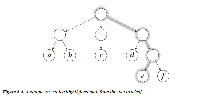
(2)树的表示 [假设要表示下面的树]

树是一种特殊的图,所以可以使用图的表示方法,但是因为树的特殊性,其实有其他更好的表示方法,最简单的就是直接用一个list即可,缺点也很明显,可读性太差了,相当不直观
T = [["a", "b"], ["c"], ["d", ["e", "f"]]]
T[2][1][0]  # 'e'
很多时候我们都能够肯定树中节点的孩子节点个数最多有多少个(比如二叉树,三叉树等等),所以比较方便的实现方式就是使用类class
# A Binary Tree Class 二叉树实例
class Tree:
    def __init__(self, left, right):
        self.left = left
        self.right = right

t = Tree(Tree("a", "b"), Tree("c", "d"))
t.right.left  # 'c'
上面的实现方式的子节点都是孩子节点,但是还有一种很常用的树的表示方式,那就是“左孩子,右兄弟”表示形式,它就适用于孩子节点数目不确定的情况
# 左孩子,右兄弟 表示方式
class Tree:
    def __init__(self, kids, next=None):
        self.kids = self.val = kids
        self.next = next
return Tree

t = Tree(Tree("a", Tree("b", Tree("c", Tree("d")))))
t.kids.next.next.val  # 'c'
[Bunch Pattern]:有意思的是,上面的实现方式使用了Python中一种常用的设计模式,叫做Bunch Pattern,貌似来自经典书籍Python Cookbook,原书介绍如下:[因为这个不太好理解和翻译,还是原文比较有味]
When prototyping (or even finalizing) data structures such as trees, it can be useful to have a flexible class that will allow you to specify arbitrary attributes in the constructor. In these cases, the “Bunch” pattern (named by Alex Martelli in the Python Cookbook) can come in handy. There are many ways of implementing it, but the gist of it is the following:
class Bunch(dict):
    def __init__(self, *args, **kwds):
        super(Bunch, self).__init__(*args, **kwds)
        self.__dict__ = self
return Bunch
There are several useful aspects to this pattern. First, it lets you create and set arbitrary attributes by supplying them as command-line arguments:
>>> x = Bunch(name="Jayne Cobb", position="Public Relations")
>>> x.name
'Jayne Cobb'
Second, by subclassing dict, you get lots of functionality for free, such as iterating over the keys/attributes or easily checking whether an attribute is present. Here’s an example:
>>> T = Bunch
>>> t = T(left=T(left="a", right="b"), right=T(left="c"))
>>> t.left
{'right': 'b', 'left': 'a'}
>>> t.left.right
'b'
>>> t['left']['right']
'b'
>>> "left" in t.right
True
>>> "right" in t.right
False
This pattern isn’t useful only when building trees, of course. You could use it for any situation where you’d want a flexible object whose attributes you could set in the constructor.
[与图有关的python模块]:
• NetworkX: http://networkx.lanl.gov
• python-graph: http://code.google.com/p/python-graph
• Graphine: http://gitorious.org/projects/graphine/pages/Home
• Pygr: a graph database http://bioinfo.mbi.ucla.edu/pygr
• Gato: a graph animation toolbox http://gato.sourceforge.net
• PADS: a collection of graph algorithms http://www.ics.uci.edu/~eppstein/PADS
5.Python编程中的一些细节
In general, the more important your program, the more you should mistrust such black boxes and seek to find out what’s going on under the cover.
作者在这里提到,如果你的程序越是重要的话,你就越是需要明白你所使用的数据结构的内部实现,甚至有些时候你要自己重新实现它。
(1)Hidden Squares 隐藏的平方运行时间
有些情况下我们可能没有注意到我们的操作是非常不高效的,例如下面的代码,如果是判断某个元素是否在list中运行时间是线性的,如果是使用set,判断某个元素是否存在只需要常数时间,所以如果我们需要判断很多元素是否存在的话,使用set的性能会更加高效。
from random import randrange
L = [randrange(10000) for i in range(1000)]
42 in L # False
S = set(L)
42 in S #False
(2)The Trouble with Floats 精度带来的烦恼
现有的计算机系统都是不能精确表达小数的![该部分内容可以阅读与计算机组成原理相关的书籍了解计算机的浮点数系统]在python中,浮点数可能带来很多的烦恼,例如,运行下面的实例,本应该是相等,但是却返回False。
sum(0.1 for i in range(10)) == 1.0 # False
**永远不要使用小数比较结果来作为两者相等的判断依据!**你最多只能判断两个浮点数在有限位数上是相等的,也就是近似相等
def almost_equal(x, y, places=7):
    return round(abs(x-y), places) == 0

almost_equal(sum(0.1 for i in range(10)), 1.0) # True
除此之外,可以使用一些有用的第三方模块,例如decimal,在需要处理金融数据的时候很有帮助
from decimal import *
sum(Decimal("0.1") for i in range(10)) == Decimal("1.0")  # Ture
还有一个有用的Sage模块,如下所示,它可以进行数学的符号运算得到准确值,如果需要也可以得到近似的浮点数解。
Sage的官方网址
sage: 3/5 * 11/7 + sqrt(5239)
13*sqrt(31) + 33/35
更多和Python中的浮点数有关的内容可以查看Floating Point Arithmetic: Issues and Limitations
问题2-12. (图的表示)
Consider the following graph representation: you use a dictionary and let each key be a pair (tuple) of two nodes, with the corresponding value set to the edge weight. For example W[u, v] = 42. What would be the advantages and disadvantages of this representation? Could you supplement it to mitigate the downsides?
The advantages and disadvantages depend on what you’re using it for. It works well for looking up edge weights efficiently but less well for iterating over the graph’s nodes or a node’s neighbors, for example. You could improve that part by using some extra structures (for example, a global list of nodes, if that’s what you need or a simple adjacency list structure, if that’s required).